Tutorials

Note

Click on the repository link to download the zip file, called tutorialData.zip, of the data you’ll need to run through the tutorials.

Make a working directory and do the tutorials in that directory.

Note

In the gif above, the working directory is located at Documents/demos/. The tutorial data files were placed in the directory called “demos.” Whatever you call it, when working in the terminal, you’ll always need to be in that directory to complete the tutorial.

The gif also showed a few commands that you may find helpful:

pwd to find the directory you’re currently in

cd to change directories

ls to list files in the folder

This tutorial builds up! Between each example and the previous examples, the new lines of code are highlighted in yellow.

Python

Python is an interpreted object oriented programming language. There is a large range of modules that are imported into python to provide extra functionality or features. pyWitness uses numpy (numerical arrays), scipy (fitting and functions), pandas (data frames), matplotlib (plotting), openpyxl (reading/writing excel), xlrd (reading/writing excel), and numba (compiler to speed up code).

Python is best started from a terminal/command prompt

ipython3 --pylab

This then lands you in a python console window

Python 3.7.9 (default, Sep  6 2020, 16:32:30)
Type 'copyright', 'credits' or 'license' for more information
IPython 7.14.0 -- An enhanced Interactive Python. Type '?' for help.

In [1]:

Commands can now be typed in to execute python and pyWitness commands. Here are some helpful tips to speed up inputing commands

Cut and paste commands (to reduce typos)

Use the command history (up and down cursor arrows) to find commands that were used previously

Use command history with search (so try import pyW and then up arrow. This will search the command history with that command fragment and probably match with a previous import pyWitness

A command can be completed by using tab. Try typing in import pyW and then pressing tab

To get help on a command, type the function and then ? for example, dp.plotROC?

Loading raw experimental data

Remember, you may need to activate pyWitness when you start a terminal by using this code

conda activate pyWitness

Start up ipython3 with

ipython3 --pylab

and pyWitness with

import pyWitness

A single Python class pyWitness.DataRaw is used to load raw data in either csv or excel format. The format of test1.csv is the same as that described in the introduction.

python
R

import pyWitness
dr = pyWitness.DataRaw("test1.csv")

pyw <- import("pyWitness")

Checking and exploring loaded data

It is useful to understand what columns and data values are stored in the raw data.

python
R

 import pyWitness
 dr = pyWitness.DataRaw("test1.csv")
 dr.checkData()

 pyw <- pyw <- import("pyWitness")
 dr <- pyw$DataRaw("./test1.csv")
 dr$checkData()

DataRaw.checkData>
DataRaw.checkData> columns      : ['Unnamed: 0' 'participantId' 'lineupSize' 'targetLineup' 'responseType' 'confidence' 'responseTime']
DataRaw.checkData> lineupSize   : [6]
DataRaw.checkData> targetLineup : ['targetAbsent' 'targetPresent']
DataRaw.checkData> responseType : ['fillerId' 'rejectId' 'suspectId']
DataRaw.checkData> confidence   : [  0  10  20  30  40  50  60  70  80  90 100]
DataRaw.checkData> number trials : 890

If the unique values for a non-mandatory column are required then this can be displayed using

python
R

import pyWitness
dr = pyWitness.DataRaw("test1.csv")
dr.columnValues("responseTime")

pyw <- import("pyWitness")
dr <- pyw$DataRaw("./test1.csv")
dr$columnValues("responseTime")

DataRaw.columnValues>           : responseTime [  1159   1296   1326 ... 161703 502420 651073]

It is possible also to load Excel files

python
R

import pyWitness
dr = pyWitness.DataRaw("test1.xlsx","test1")

pyw <- import("pyWitness")
dr <- pyw$DataRaw("test1.xlsx","test1")

The second argument is the sheet name within the workbook (in the example above, it’s “test1”).

Processing raw experimental data

To process the raw data the function pyWitness.DataRaw.process needs to be called on a raw data object. This calculates the cumulative rates from the raw data.

python
R

import pyWitness
dr = pyWitness.DataRaw("test1.csv")
dp = dr.process()

pyw <- import("pyWitness")
dr <- pyw$DataRaw("./test1.csv")
dp <- dr$process()

Once pyWitness.DataRaw.process is called two DataFrames are created. One contains a pivot table and the other contains rates.

python
R

import pyWitness
dr = pyWitness.DataRaw("test1.csv")
dp = dr.process()
dp.printPivot()
dp.printRates()

pyw <- import("pyWitness")
dr <- pyw$DataRaw("./test1.csv")
dp <- dr$process()
dp$printPivot()
dp$printRates()

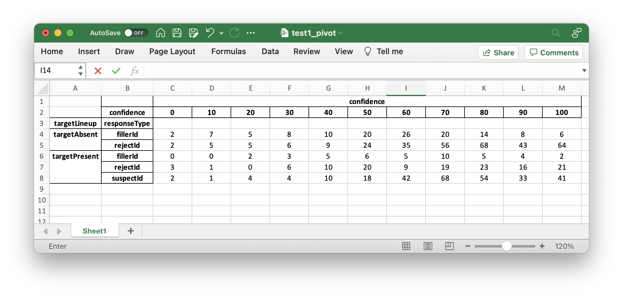
You should see the following output of the dp.printPivot().

                          confidence
confidence                        0    10   20   30    40    50    60    70    80    90    100
targetLineup  responseType
targetAbsent  fillerId            2.0  7.0  5.0  8.0  10.0  20.0  26.0  20.0  14.0   8.0   6.0
              rejectId            2.0  5.0  5.0  6.0   9.0  24.0  35.0  56.0  68.0  43.0  64.0
targetPresent fillerId            0.0  0.0  2.0  3.0   5.0   6.0   5.0  10.0   5.0   4.0   2.0
              rejectId            3.0  1.0  0.0  6.0  10.0  20.0   9.0  19.0  23.0  16.0  21.0
              suspectId           2.0  1.0  4.0  4.0  10.0  18.0  42.0  68.0  54.0  33.0  41.0
total number of participants 890.0

In the output above are frequencies by confidence levels for each response type. To familiarize you with the output, in the table above, 8 filler identifications were given with 30% confidence on the target-absent lineups, 64 reject identifications (i.e., “The perp is not in the lineup”) given with 100% confidence on the target-absent lineups, and 41 guilty suspect identifications (from target-present lineups) given with 100% confidence.

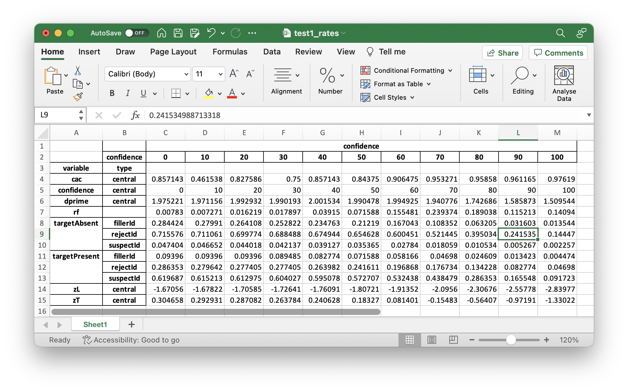
You should also see the following output for dp.printRates()

                    confidence
confidence                     0          10         20         30         40         50         60         70         80         90          100
variable      type
cac           central     0.857143   0.461538   0.827586   0.750000   0.857143   0.843750   0.906475   0.953271   0.958580   0.961165    0.976190
confidence    central     0          10         20         30         40         50         60         70         80             90          100
dprime        central     1.975221   1.971156   1.992932   1.990193   2.001534   1.990478   1.994925   1.940776   1.742686   1.585873    1.509544
rf                        0.007830   0.007271   0.016219   0.017897   0.039150   0.071588   0.155481   0.239374   0.189038   0.115213    0.140940
targetAbsent  fillerId    0.284424   0.279910   0.264108   0.252822   0.234763   0.212190   0.167043   0.108352   0.063205   0.031603    0.013544
              rejectId    0.715576   0.711061   0.699774   0.688488   0.674944   0.654628   0.600451   0.521445   0.395034   0.241535    0.144470
              suspectId   0.047404   0.046652   0.044018   0.042137   0.039127   0.035365   0.027840   0.018059   0.010534   0.005267    0.002257
targetPresent fillerId    0.093960   0.093960   0.093960   0.089485   0.082774   0.071588   0.058166   0.046980   0.024609   0.013423    0.004474
              rejectId    0.286353   0.279642   0.277405   0.277405   0.263982   0.241611   0.196868   0.176734   0.134228   0.082774    0.046980
              suspectId   0.619687   0.615213   0.612975   0.604027   0.595078   0.572707   0.532438   0.438479   0.286353   0.165548    0.091723
zL            central    -1.670562  -1.678225  -1.705849  -1.726409  -1.760906  -1.807208  -1.913524  -2.095603  -2.306755  -2.557781   -2.839765
zT            central     0.304658   0.292931   0.287082   0.263784   0.240628   0.183270   0.081401  -0.154827  -0.564069  -0.971908   -1.330222

In the table above, the overall false ID rate is 0.047, the overall correct ID rate is 0.620, and the overall correct rejection rate is 0.716.

Note

In the example there is no suspectId for targetAbsent lineups. Here the targetAbsent.suspectId is estimated as targetAbsent.fillerId/lineupSize

To see overall descriptive statistics, use

python
R

import pyWitness
dr = pyWitness.DataRaw("test1.csv")
dp = dr.process()
dp.printDescriptiveStats()

pyw <- import("pyWitness")
dr <- pyw$DataRaw("./test1.csv")
dp <- dr$process()
dp$printDescriptiveStats()

and you’ll see this output:

Number of lineups                    890.0
Number of target-absent lineups      443.0
Number of target-present lineups     447.0
Correct ID rate                        0.6196868008948546
False ID rate                          0.0474040632054176
dPrime                                 1.9752208100241062
pAUC                                   0.02066155955774986

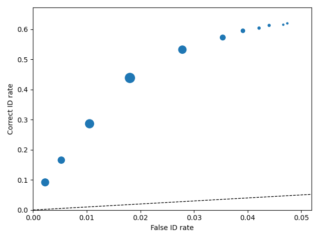
Plotting ROC curves

python
R

 import pyWitness
 dr = pyWitness.DataRaw("test1.csv")
 dp = dr.process()
 dp.plotROC()

 pyw <- import("pyWitness")
 dr <- pyw$DataRaw("./test1.csv")
 dp <- dr$process()
 dp$plotROC()
 mpl$pyplot$show()

Note

The symbol size is the relative frequency and can be changed by setting dp.plotROC(relativeFrequencyScale = 400)

Note

The transparency of the plot can be changed by setting alpha in the plot command, so dp.plotROC(alpha = 0.5)

The black dashed line in the plot represents chance performance.

Plotting CAC curves

python
R

import pyWitness
dr = pyWitness.DataRaw("test1.csv")
dp = dr.process()
dp.plotCAC()

pyw <- import("pyWitness")
dr <- pyw$DataRaw("./test1.csv")
dp <- dr$process()
dp$plotCAC()
mpl$pyplot$show()

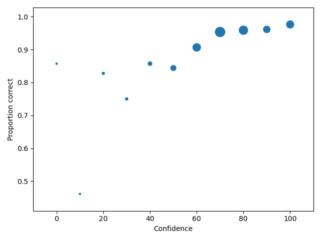
Note

The transparency of the plot can be changed by setting alpha in the plot command, so dp.plotCAC(alpha = 0.5)

Warning

To plot CAC curves with different target-present base rates, the base rate needs to be given to the process function of DataRaw, for example, dp = dr.process(baseRate=0.2)

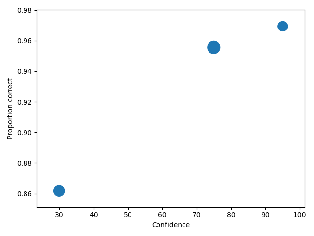
Collapsing the categorical data

The dataset used in this tutorial has 11 confidence levels (0, 10, 20, 30, 40, 50, 60, 70, 80, 90 and 100). Often confidence levels need to be binned or collapsed. This is best performed on the raw data before calling process(). This is done with the collapseCategoricalData method of DataRaw, and shown in example below, where the new bins are (0-60 map to 30, 70-80 to 75 and 90-100 to 95).

python
R

import pyWitness
dr = pyWitness.DataRaw("test1.csv")
dr.collapseCategoricalData(column='confidence',
                       map={0: 30, 10: 30, 20: 30, 30: 30, 40: 30, 50: 30, 60: 30,
                            70: 75, 80: 75,
                            90: 95, 100: 95})
dp = dr.process()
dp.plotCAC()

pyw <- import("pyWitness")
dr <- pyw$DataRaw("./test1.csv")
dr$collapseCategoricalData(column='confidence',map=list("0"=30, "10"=30, "20"=30, "30"=30,
                                                        "40"=30,"50"=30, "60"=30,"70"=75, "80"=75,"90"=95, "100"=95))
dp <- dr$process()
dp$plotCAC()
mpl$pyplot$show()

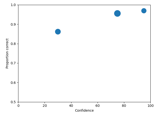
To rescale the axes, you can use

python
R

import matplotlib as _plt
xlim(0,100)
ylim(0.50,1.0)

pyw <- import("pyWitness")
dr <- pyw$DataRaw("./test1.csv")
dr$collapseCategoricalData(column='confidence',map=list("0"=30, "10"=30, "20"=30, "30"=30,               "40"=30,"50"=30, "60"=30,"70"=75, "80"=75,"90"=95, "100"=95))
dp <- dr$process()
dp$plotCAC()
invisible(mpl$pyplot$ylim(0.50,1.0))
mpl$pyplot$show()

and you get

Note

If you err, the collapseCategoricalData the data might be inconsistent. To start with the original data so call collapseCategoricalData with reload=True

Collapsing (binning) continuous data

Some data are not categorical variables, but continuous variables.

python
R

import pyWitness
dr = pyWitness.DataRaw("test1.csv")
dr.collapseContinuousData(column = "confidence",bins = [-1,60,80,100],labels= [1,2,3])
dp = dr.process()
dp.plotROC()

 pyw <- import("pyWitness")
 dr <- pyw$DataRaw("./test1.csv")
 dr$collapseContinuousData(column = "confidence", bins = c(-1,60,80,100),labels= c(1,2,3))
 dp <- dr$process()
 dp$plotROC()
 mpl$pyplot$show()

Note

labels=None can be used and the bins will be automatically labelled

Note

The bin edges are exclusive of the low edge and inclusive of the high edge

Warning

Confidence needs to be a numerical value because ROC analysis requires a value that can be ordered.

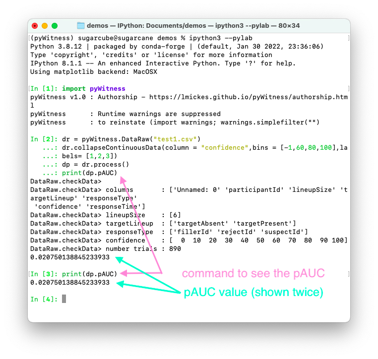
Calculating pAUC and performing statistical tests

pAUC is calculated when dr.process() is called. Simpson’s rule integrates the area under the ROC curve up to a maximum value. If the maximum value is between two data points, linear interpolation is used to calculate the most liberal point (i.e., the lowest level of confidence).

python
R

import pyWitness
dr = pyWitness.DataRaw("test1.csv")
dr.collapseContinuousData(column = "confidence",bins = [-1,60,80,100],labels= [1,2,3])
dp = dr.process()
print(dp.pAUC)

pyw <- import("pyWitness")
dr <- pyw$DataRaw("./test1.csv")
dr$collapseContinuousData(column = "confidence",bins = c(-1,60,80,100),labels= c(1,2,3))
dp <- dr$process()
print(dp$pAUC)

Data-model ROC comparision for test1.csv

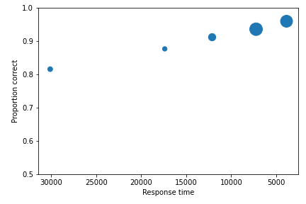
Plotting RAC curves

To perform analyses with a different variable than confidence, for example, response time, use the following code. The important change is highlighted.

python
R

 import pyWitness
 drRAC = pyWitness.DataRaw("test1.csv")
 drRAC.collapseContinuousData(column="responseTime",bins=[0, 5000, 10000, 15000, 20000, 99999],labels=[1, 2, 3, 4, 5])
 dpRAC = drRAC.process(reverseConfidence=True,dependentVariable="responseTime")
 dpRAC.plotCAC()

pyw <- import("pyWitness")
drRAC <- pyw$DataRaw("./test1.csv")
drRAC$collapseContinuousData(column="responseTime",
             bins=c(0, 5000, 10000, 15000, 20000, 99999),labels=c(1, 2, 3, 4, 5))
dpRAC <- drRAC$process(reverseConfidence=TRUE,dependentVariable="responseTime")
dpRAC$plotCAC()
invisible(mpl$pyplot$xlabel("Response Time"))
invisible(mpl$pyplot$ylim(.50,1.0))
invisible(mpl$pyplot$savefig("test1RAC.png"))
invisible(mpl$pyplot$savefig("test1RAC.pdf"))

The plot will look like this:

Fitting signal detection-based models to data

There are many models available in pyWitness. We’ll start with the independent observation model. To load and process the data is the same as before (lines 1-4), the fitting part is new and the code is highlighted (lines 5-7).

python
R

import pyWitness
dr = pyWitness.DataRaw("test1.csv")
dr.collapseContinuousData(column = "confidence",bins = [-1,60,80,100],labels= [1,2,3])
dp = dr.process()
mf = pyWitness.ModelFitIndependentObservation(dp)
mf.setEqualVariance()
mf.fit()

pyw <- import("pyWitness",convert=TRUE)
dr <- pyw$DataRaw("./test1.csv")
dr$collapseContinuousData(column = "confidence",bins = c(-1,60,80,100),labels= c(1,2,3))
dp <- dr$process()
mf <- pyw$ModelFitIndependentObservation(dp)
mf$setEqualVariance()
mf$fit()

Line 5 constructs a fit object, line 6 sets the model parameters to equal variance and line 7 starts the minimiser. The output from the fit (execution of line 7) is something like the following

fit iterations 223
fit status     Optimization terminated successfully.
fit time       9.376720442
fit chi2       10.300411274463407
fit ndf        4
fit chi2/ndf   2.5751028186158518
fit p-value    0.035660197825222784

To clearly see how the fitting works, the following code is the same as above but with mf.printParameters() on lines 6, 9, and 12.

python
R

import pyWitness
dr = pyWitness.DataRaw("test1.csv")
dr.collapseContinuousData(column = "confidence",bins = [-1,60,80,100],labels= [1,2,3])
dp = dr.process()
mf = pyWitness.ModelFitIndependentObservation(dp)
mf.printParameters()

mf.setEqualVariance()
mf.printParameters()

mf.fit()
mf.printParameters()

pyw <- import("pyWitness")
dr <- pyw$DataRaw("./test1.csv")
dr$collapseContinuousData(column = "confidence",bins = c(-1,60,80,100),labels= c(1,2,3))
dp <- dr$process()
mf <- pyw$ModelFitIndependentObservation(dp)
mf$printParameters()

mf$setEqualVariance()
mf$printParameters()

mf$fit()
mf$printParameters()

After creating the mf object (line 9) the parameters are at their default values and free

lureMean 0.0 (free)
lureSigma 1.0 (free)
targetMean 1.0 (free)
targetSigma 1.0 (free)
lureBetweenSigma 0.0 (free)
targetBetweenSigma 0.0 (free)
c1 1.0 (free)
c2 1.5 (free)
c3 2.0 (free)

Typically you would want to control the fit parameters. setEqualVariance sets some default model which is an appropriate start; line 12 yields

lureMean 0.0 (fixed)
lureSigma 1.0 (fixed targetSigma)
targetMean 1.0 (free)
targetSigma 1.0 (fixed)
lureBetweenSigma 0.3 (fixed targetBetweenSigma)
targetBetweenSigma 0.3 (free)
c1 1.0 (free)
c2 1.5 (free)
c3 2.0 (free)

Comparing these two fit parameters settings

lureSigma is forced to be equal to targetSigma

targetSigma is fixed to its current value

lureBetweenSigma is fixed to targetBetweenSigma

targetBetweenSigma is fixed to its current value

After running the fit the parameters are updated so the output of line 12 in the code example gives

ModelFit.printParameters>  lureMean 0.000 (fixed)
ModelFit.printParameters>  lureSigma 1.000 (fixed targetSigma)
ModelFit.printParameters>  targetMean 1.798 (free)
ModelFit.printParameters>  targetSigma 1.000 (fixed)
ModelFit.printParameters>  lureBetweenSigma 0.605 (fixed targetBetweenSigma)
ModelFit.printParameters>  targetBetweenSigma 0.605 (free)
ModelFit.printParameters>  c1 1.402 (free)
ModelFit.printParameters>  c2 1.935 (free)
ModelFit.printParameters>  c3 2.677 (free)

There many ways to control the model

Parameter control examples
Command	Notes
`mf.lureMean.value = -0.1`	Sets the lure mean parameter to -0.1
`mf.targetMean.fixed = True`	Fixed the parameter so it cannot change during a fit
`mf.lureMean.fixed = False`	Unfixes the parameter so it will be free in a fit
`mf.c1.set_equal(mf.c2)`	Locks `c1` and `c2` together
`mf.lureBetweenSigma.unset_equal()`	Release the linking of lureBetweenSigma and targetBetweenSigma

There are multiple fits available and they all have the same interface but differ in the construction line

python
R

dr = pyWitness.DataRaw("test1.csv")
dr.collapseContinuousData(column="confidence")
dp = dr.process()

mf_io = pyWitness.ModelFitIndependentObservation(dp)
mf_br = pyWitness.ModelFitBestRest(dp)
mf_en = pyWitness.ModelFitEnsemble(dp)
mf_in = pyWitness.ModelFitIntegration(dp)

pyw <- import("pyWitness")
dr <- pyw$DataRaw("./test1.csv")
dp <- dr$process()

mf_io <- pyw$ModelFitIndependentObservation(dp)
mf_br <- pyw$ModelFitBestRest(dp)
mf_en <- pyw$ModelFitEnsemble(dp)
mf_in <- pyw$ModelFitIntegration(dp)

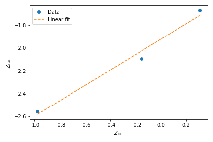
Setting initial fit parameters

With data samples with large number of confidence bins the fits can take a large number of iterations to converge (long run times). Sensible fit parameters can be be estimated from the data.

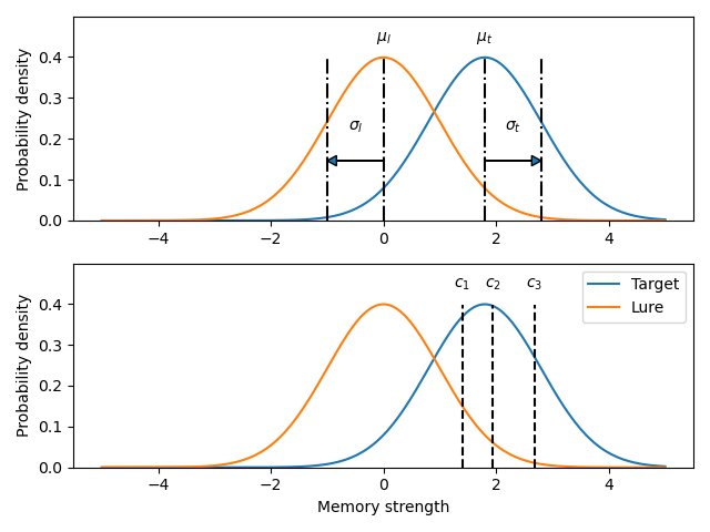
To estimate the target mean \(\mu_t\) and sigma \(\sigma_t\) the following relation is used

\[Z(R_{T,i}) = \frac{Z(R_{L,i})- \mu_t}{\sigma_t}\]

Rearranging gives

\[\sigma_t Z(R_{T,i}) = Z(R_{L,i}) - \mu_s\]

There is a linear relationship between target and lure \(Z\) values. This can be plotted and a linear fit used to estimate the gradient and intercept.

python
R

import pyWitness
dr = pyWitness.DataRaw("test1.csv")
dr.collapseContinuousData(column = "confidence",bins = [-1,60,80,100],labels= [1,2,3])
dp = dr.process()
dp.plotHitVsFalseAlarmRate()

pyw <- import("pyWitness")
dr <- pyw$DataRaw("./test1.csv")
dr$collapseContinuousData(column = "confidence",bins = c(-1,60,80,100),labels = c(1,2,3))
dp <- dr$process()
dp$plotHitVsFalseAlarmRate()
invisible(mpl$pyplot$savefig("HvFA.png"))

Hit rate vs. false alarm rate for test1.csv

python
R

import pyWitness
dr = pyWitness.DataRaw("test1.csv")
dr.collapseContinuousData(column = "confidence",bins = [-1,60,80,100],labels= [1,2,3])
dp = dr.process()
mf = pyWitness.ModelFitIndependentObservation(dp)
mf.printParameters()

mf.setEqualVariance()
mf.setParameterEstimates()
mf.printParameters()

mf.fit()
mf.printParameters()

pyw <- import("pyWitness")
dr <- pyw$DataRaw("./test1.csv")
dr$collapseContinuousData(column = "confidence",bins = c(-1,60,80,100),labels = c(1,2,3))
dp <- dr$process()
mf <- pyw$ModelFitIndependentObservation(dp)

mf$setEqualVariance()
mf$setParameterEstimates()
mf$printParameters()

mf$fit()
mf$printParameters()

Plotting fit and models

It is important to understand the performance of a given particular fit. The following plot compares the experimental data to the model fit.

python
R

import pyWitness
dr = pyWitness.DataRaw("test1.csv")
dr.collapseContinuousData(column = "confidence",bins = [-1,60,80,100],labels= None)
dp = dr.process()
dp.calculateConfidenceBootstrap(nBootstraps=200)
mf = pyWitness.ModelFitIndependentObservation(dp)
mf.setEqualVariance()
mf.fit()

pyw <- import("pyWitness")
dr <- pyw$DataRaw("./test1.csv")
dr$collapseContinuousData(column = "confidence",bins = c(-1,60,80,100),labels = c(1,2,3))
dp <- dr$process()
dp$calculateConfidenceBootstrap(nBootstraps=as.integer(200))
mf <- pyw$ModelFitIndependentObservation(dp)
mf$setEqualVariance()
mf$fit()

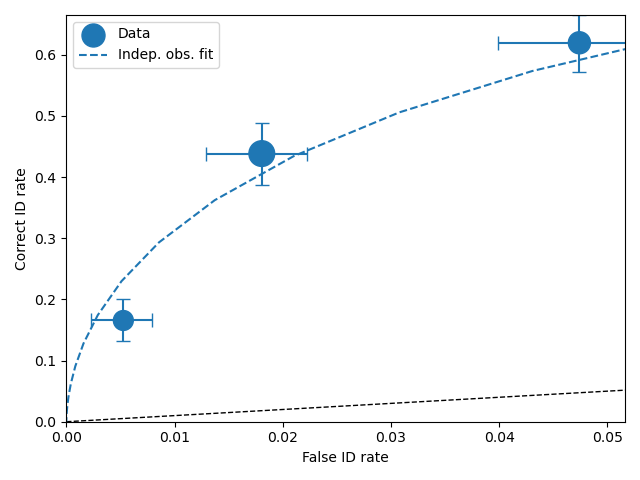
To compare an ROC plot between data and fit

python
R

dp.plotROC(label="Data")
mf.plotROC(label="Indep. obs. fit")

import matplotlib.pyplot as _plt
_plt.legend()

pyw <- import("pyWitness")
dr <- pyw$DataRaw("./test1.csv")
dr$collapseContinuousData(column = "confidence",bins = c(-1,60,80,100),labels = c(1,2,3))
dp <- dr$process()
dp$calculateConfidenceBootstrap(nBootstraps=as.integer(200))
mf <- pyw$ModelFitIndependentObservation(dp)
mf$setEqualVariance()
mf$fit()
dp$plotROC(label="Data")
mf$plotROC(label="Indep. obs. fit")
mpl$pyplot$legend()
mpl$pyplot$show()

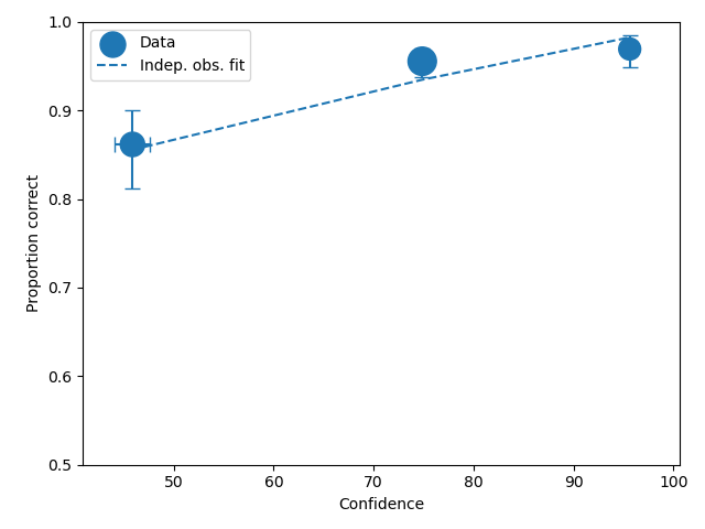
To compare a CAC plot between data and fit

python
R

dp.plotCAC(label="Data")
mf.plotCAC(label="Indep. obs. fit")

import matplotlib.pyplot as _plt
_plt.legend()

dp$plotCAC(label="Data")
mf$plotCAC(label="Indep. obs. fit")

mpl$pyplot$legend()

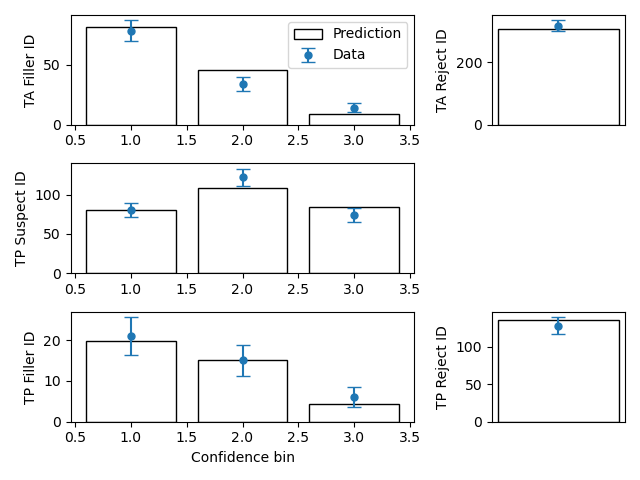
Data-model CAC comparision for test1.csv

To compare frequencies in each bin between data and fit

python
R

mf.plotFit()

mf$plotFit()

Once a fit has been performed, the model can be displayed as a function of memory strength and includes the lure and target distributions with means and standard deviations (top panel of plot below) and the associated criteria, c1 (low confidence), c2 (medium confidence), and c3 (high confidence) (bottom panel of plot below). This simple command belonging to a ModelFit object can be used to make the plot below.

python
R

mf.plotModel()

mf$plotModel()

d-prime calculation

The d-prime can be calculated by computing

\[d^{\prime} = Z(R_{T,i}) - Z(R_{L,i})\]

where \(R_{T,i}\) is the cumulative rate for targets (\(T\)) with confidence \(i\), \(R_{L,i}\) is the cumulative rate for lures (\(L\)) with confidence \(i\) and \(Z\) is the inverse normal CDF. This can be evaluated for every confidence bin, but there are conventions for lineups and showups. For all confidence levels \(d^{\prime}\) is stored in the rates dataframe, so dp.printRates() gives

                           confidence
confidence                          3          2          1
targetLineup  responseType
cac           central        0.956357   0.940618   0.839228
confidence    central       95.588235  74.859335  44.778068
dprime        central        1.433207   1.748223   1.767339
rf                           0.264691   0.422903   0.312406
targetAbsent  fillerId       0.044660   0.141748   0.335922
              rejectId       0.217476   0.473786   0.664078
              suspectId      0.007443   0.023625   0.055987
targetPresent fillerId       0.018832   0.080979   0.152542
              rejectId       0.080979   0.163842   0.276836
              suspectId      0.158192   0.406780   0.570621

A member variable dPrime in DataProcessed is set according to

Lineup convention \(d^{\prime}\) is the lowest confidence (most liberal) so dp.dPrime is 1.767339
Showup convention \(d^{\prime}\) is the lowest positive confidence

\(d\) can also be calculated from a signal detection model so

\[d = \frac{\mu_{T} - \mu_{L}}{ \sqrt{\frac{\sigma_T^2 + \sigma_L^2}{2}} }\]

This is calculated from the fit parameters for the fits described in the previous section so

In [X]: mf.d
Out[X]: 1.7976601843420954

Writing results to file

The internal dataframes can be written to either csv or xlsx file format for further analysis. There are four functions belonging to DataProcessed.

writePivotExcel writes the pivot table to excel

writePivotCsv writes the pivot table to csv

writeRatesExcel writes the cummulative rates table to excel

writeRatesCsv writes the cummulative rates table to csv

The string argument for the functions is the file name.

python
R

import pyWitness
dr = pyWitness.DataRaw("test1.csv")
dp = dr.process()
dp.writePivotExcel("test1_pivot.xlsx")
dp.writePivotCsv("test1_pivot.csv")
dp.writeRatesExcel("test1_rates.xlsx")
dp.writeRatesCsv("test1_rates.csv")

 pyw <- import("pyWitness")
 dr <- pyw$DataRaw("./test1.csv")
 dp <- dr$process()
 dp$writePivotExcel("./test1_pivot.xlsx")
 dp$writePivotCsv("./test1_pivot.csv")
 dp$writeRatesExcel("./test1_rates.xlsx")
 dp$writeRatesCsv("./test1_rates.csv")

Designated innocent suspect in target absent (TA) lineups

In TA lineups the suspect ID rate is estimated as the fillerID/lineupSize. In some experiments a designated innocent suspect is used. This is possible with pyWitness.

The raw data in the responseType column will have an extra possible type called designateId

Then all of the analyses will proceed normally, but now the targetAbsent suspectId row will be populated with data from the designated innocent suspect

Sometimes it is useful to check if raw data contains designateId, this is done by calling dataRaw.isDesignateId

To convert all designateId to fillerIds one must call dataRaw.removeDesignates()