Advanced tutorials

Bootstrapping uncertainties/confidence limits

To create confidence limits on binned cumulative, statistical measures and parameters, pyWitness uses the bootstrap method. This method takes \(N\) random participants from the original data with replacement. pyWitness can then proceed to compute any quantity (ROC, CAC, pAUC, fit parameters). This is repeated \(M\) times and the distribution of the computed quantity used to calculate a confidence interval with a user definable range.

• python
• R

import pyWitness
dr = pyWitness.DataRaw("test1.csv")
dp = dr.process()
dp.calculateConfidenceBootstrap(nBootstraps=200, cl=95)
dp.printRates()

pyw <- import("pyWitness")
dr <- pyw$DataRaw("./test1.csv")
dr$collapseContinuousData(column = "confidence",bins = c(-1,60,80,100),labels=py_none())
dp <- dr$process()
dp$calculateConfidenceBootstrap(nBootstraps=as.integer(200), cl=95)
dp$printRates()

After calling calculateConfidenceBootstrap the rates table is populated with the 95% confidence limit data

                                      confidence
confidence                            1          2          3
variable      type
cac           central          0.861702   0.955614   0.969432
              high             0.898148   0.969998   0.982672
              low              0.819782   0.934552   0.946858
confidence    central         45.873016  74.866469  95.630252
              high            47.962794  75.440947  96.258406
              low             44.128214  74.301501  94.949277
dprime        central          1.975221   1.940776   1.585873
              high             2.120760   2.101158   1.834337
              low              1.815447   1.753813   1.328038
rf                             0.315436   0.428412   0.256152
targetAbsent  fillerId         0.284424   0.108352   0.031603
              fillerId_high    0.321175   0.134259   0.048269
              fillerId_low     0.240872   0.082314   0.016915
              rejectId         0.715576   0.521445   0.241535
              rejectId_high    0.752949   0.560668   0.277414
              rejectId_low     0.672739   0.472804   0.202311
              suspectId        0.047404   0.018059   0.005267
              suspectId_high   0.053529   0.022377   0.008045
              suspectId_low    0.040145   0.013719   0.002819
targetPresent fillerId         0.093960   0.046980   0.013423
              fillerId_high    0.118805   0.067776   0.024778
              fillerId_low     0.067489   0.025640   0.002278
              rejectId         0.286353   0.176734   0.082774
              rejectId_high    0.329399   0.211019   0.106384
              rejectId_low     0.238167   0.140321   0.055782
              suspectId        0.619687   0.438479   0.165548
              suspectId_high   0.668216   0.493503   0.196507
              suspectId_low    0.567298   0.392393   0.128108
zL            central         -1.670562  -2.095603  -2.557781
              high            -1.611559  -2.006968  -2.406877
              low             -1.749027  -2.205230  -2.768544
zT            central          0.304658  -0.154827  -0.971908
              high             0.434992  -0.016287  -0.854162
              low              0.169499  -0.273088  -1.135387

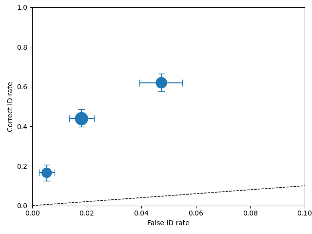
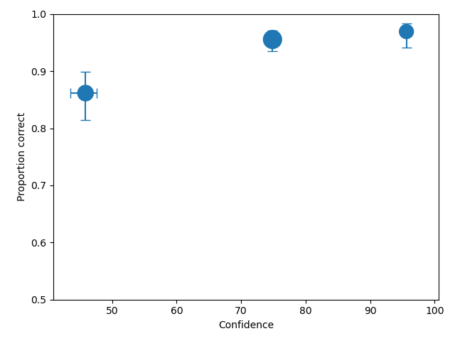
If a plot function (plotROC, plotCAC) is callled after calling calculateConfidenceBootstrap then the confidence interval is drawn as error bars, as shown in the ROC plot and CAC plot, respectively, below.

• python
• R

import pyWitness
dr = pyWitness.DataRaw("test1.csv")
dp = dr.process()
dp.calculateConfidenceBootstrap(nBootstraps=200, cl=95)
dp.plotROC()

pyw <- import("pyWitness")
dr <- pyw$DataRaw("./test1.csv")
dr$collapseContinuousData(column = "confidence",bins = c(-1,60,80,100),labels=py_none())
dp <- dr$process()
dp$calculateConfidenceBootstrap(nBootstraps=as.integer(200), cl=95)
dp$plotROC()

• python
• R

import pyWitness
dr = pyWitness.DataRaw("test1.csv")
dp = dr.process()
dp.calculateConfidenceBootstrap(nBootstraps=200, cl=95)
dp.plotCAC()

pyw <- import("pyWitness")
dr <- pyw$DataRaw("./test1.csv")
dr$collapseContinuousData(column = "confidence",bins = c(-1,60,80,100),labels=py_none())
dp <- dr$process()
dp$calculateConfidenceBootstrap(nBootstraps=as.integer(200), cl=95)
dp$plotCAC()

Loading raw data excel format

If the file is in excel format you will need to specify which sheet the raw data is stored in

• python
• R

import pyWitness
dr = pyWitness.DataRaw("test2.xlsx",excelSheet = "raw data")

pyw <- import("pyWitness")
dr <- pyw$DataRaw("./test2.xlsx",excelSheet = "raw data")

Transforming data into common format

The raw experimental data does not have to be in the internal format used by pyWitness. As the data is loaded is it possible to replace the name of the data columns and the values stored.

• python
• R

import pyWitness
dr = pyWitness.DataRaw("test2.csv",
                       dataMapping = {"lineupSize":"lineup_size",
                                      "targetLineup":"culprit_present",
                       "targetPresent":"present",
                       "targetAbsent":"absent",
                       "responseType":"id_type",
                       "suspectId":"suspect",
                       "fillerId":"filler",
                       "rejectId":"reject",
                       "confidence":"conf_level"}))

pyw <- import("pyWitness")
dr <- pyw$DataRaw("./test2.csv",
                        dataMapping = list("lineupSize"="lineup_size",
                                       "targetLineup"="culprit_present",
                                       "targetPresent"="present",
                                       "targetAbsent"="absent",
                                       "responseType"="id_type",
                                       "suspectId"="suspect",
                                       "fillerId"="filler",
                                       "rejectId"="reject",
                                       "confidence"="conf_level"))

Processing data for two conditions

A single data file might have different experimental condtions. Imagine your data file has a column labelled Condition and the values for each participant is either Control or Verbal. To proccess only the Control participants the following options are required for DataRaw.process()

• python
• R

import pyWitness
dr = pyWitness.DataRaw("test2.csv")
dr.cutData(column="previouslyViewedVideo",value=1,option="keep")
dpControl = dr.process(column="group", condition="Control")

pyw <- import("pyWitness")
dr <- pyw$DataRaw("./test2.csv")
dr$cutData(column="previouslyViewedVideo",value=1,option="keep")
dpControl = dr$process(column="group", condition="Control")

If you have a file with multiple conditions it is straightforward to make multiple DataProcessed for each condition, as in the following

• python
• R

import pyWitness
dr = pyWitness.DataRaw("test2.csv")
dr.cutData(column="previouslyViewedVideo",value=1,option="keep")
dpControl = dr.process(column="group", condition="Control")
dpVerbal = dr.process(column="group", condition="Verbal")

pyw <- import("pyWitness")
dr <- pyw$DataRaw("./test2.csv")
dr$cutData(column="previouslyViewedVideo",value=1,option="keep")
dpControl <- dr$process(column="group", condition="Control")
dpVerbal <- dr$process(column="group", condition="Verbal")

Statistical (pAUC) comparision between two conditions

One way to compare pAUC values of two conditions is use the following code on the test2 data. You can check out the script we wrote called pAUCexample.py.

• python
• R

import pyWitness
dr = pyWitness.DataRaw("test2.csv")
dr.cutData(column="previouslyViewedVideo",value=1,option="keep")
dpControl = dr.process(column="group", condition="Control")
dpVerbal = dr.process(column="group", condition="Verbal")

pyw <- import("pyWitness")
dr <- pyw$DataRaw("./test2.csv")
dr$cutData(column="previouslyViewedVideo",value=1,option="keep")
dpControl <- dr$process(column="group", condition="Control")
dpVerbal <- dr$process(column="group", condition="Verbal")

To find the lowest false ID rate from both conditions,

• python
• R

import pyWitness
dr = pyWitness.DataRaw("test2.csv")
dr.cutData(column="previouslyViewedVideo",value=1,option="keep")
dpControl = dr.process(column="group", condition="Control")
dpVerbal = dr.process(column="group", condition="Verbal")
minRate = min(dpControl.liberalTargetAbsentSuspectId,dpVerbal.liberalTargetAbsentSuspectId)

pyw <- import("pyWitness")
dr <- pyw$DataRaw("./test2.csv")
dr$cutData(column="previouslyViewedVideo",value=1,option="keep")
dpControl <- dr$process(column="group", condition="Control")
dpVerbal <- dr$process(column="group", condition="Verbal")
minRate <- min(dpControl$liberalTargetAbsentSuspectId,dpVerbal$liberalTargetAbsentSuspectId)

You have to process the data again, with this minRate

• python
• R

import pyWitness
dr = pyWitness.DataRaw("test2.csv")
dr.cutData(column="previouslyViewedVideo",value=1,option="keep")
dpControl = dr.process(column="group", condition="Control")
dpVerbal = dr.process(column="group", condition="Verbal")
minRate = min(dpControl.liberalTargetAbsentSuspectId,dpVerbal.liberalTargetAbsentSuspectId)
dpControl = dr.process("group","Control",pAUCLiberal=minRate)
dpControl.calculateConfidenceBootstrap(nBootstraps=200)
dpVerbal = dr.process("group","Verbal",pAUCLiberal=minRate)
dpVerbal.calculateConfidenceBootstrap(nBootstraps=200)
dpControl.comparePAUC(dpVerbal)

pyw <- import("pyWitness")
dr <- pyw$DataRaw("./test2.csv")
dr$cutData(column="previouslyViewedVideo",value=1,option="keep")
dpControl = dr$process(column="group", condition="Control")
dpVerbal = dr$process(column="group", condition="Verbal")
minRate = min(dpControl$liberalTargetAbsentSuspectId,dpVerbal$liberalTargetAbsentSuspectId)
dpControl = dr$process("group","Control",pAUCLiberal=minRate)
dpControl$calculateConfidenceBootstrap(nBootstraps=as.integer(200))
dpVerbal = dr$process("group","Verbal",pAUCLiberal=minRate)
dpVerbal$calculateConfidenceBootstrap(nBootstraps=as.integer(200))
dpControl$comparePAUC(dpVerbal)

To plot the ROC curves, use DataProcess.plotROC

• python
• R

dpControl.plotROC(label = "Control data", relativeFrequencyScale=400)
dpVerbal.plotROC(label = "Verbal data", relativeFrequencyScale=400)

dpControl$plotROC(label = "Control data", relativeFrequencyScale=400)
dpVerbal$plotROC(label = "Verbal data", relativeFrequencyScale=400)

Note

The symbol size is the relative frequency and can be changed by setting dp.plotROC(relativeFrequencyScale = 400)

And your plot will look like this one:

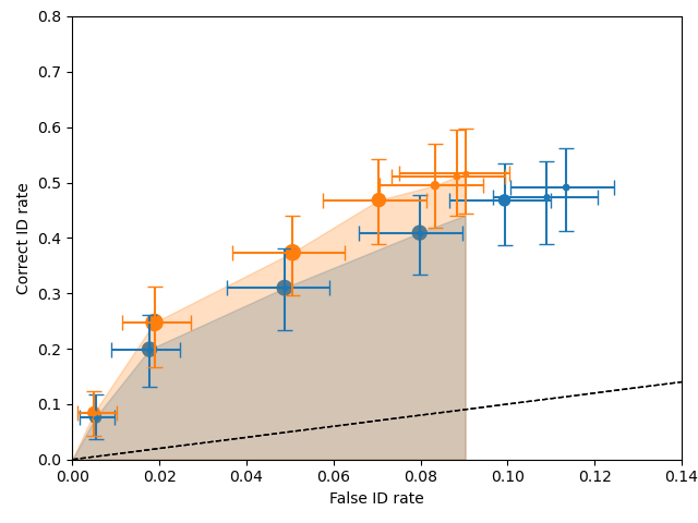
The shaded regions are the pAUCs that were compared. You can see that they both used the same minimum false ID rate. The error bars are 95% confidence intervals. The dashed black line represents chance performance.

Note

The uncertainities can be changed by setting them to .68, for example dpControl.calculateConfidenceBootstrap(nBootstraps=200,cl=68) and dpVerbal.calculateConfidenceBootstrap(nBootstraps=200,cl=68)

Loading processed data

You might already have processed the raw data, or you only have a table of data. It is possible to load a file to perform model fits etc. The processed data need to be in the following CSV format. This is basically the same format as the pivot table stored in DataProcessed.

Processed data columns and allowed values

confidence	0	10	20	30	40	50	60	70	80	90	100
targetAbsent fillerId	2	7	5	8	10	20	26	20	14	8	6
targetAbsent rejectId	2	5	5	6	9	24	35	56	68	43	64
targetPresent fillerId	0	0	2	3	5	6	5	10	5	4	2
targetPresent rejectId	3	1	0	6	10	20	9	19	23	16	21
targetPresent suspectId	2	1	4	4	10	18	43	68	54	33	41

Note

If the targetAbsent suspectId row is not present it is estimated by (targetAbsent fillerId)/lineupSize

The data are stored in data/tutorials/test1_processed.csv

• python
• R

import pyWitness
dp = pyWitness.DataProcessed("test1_processed.csv", lineupSize = 6)

pyw <- import("pyWitness")
dp = pyw$DataProcessed("./test1_processed.csv", lineupSize = 6)

Using instances of raw data, processed data and model fits

Using an object orientated approach allows multiple instances (objects) to be created and manipulated. This allows many different data file variations on the processed data and model fits to be manipulated simultanuously in a single Python session.

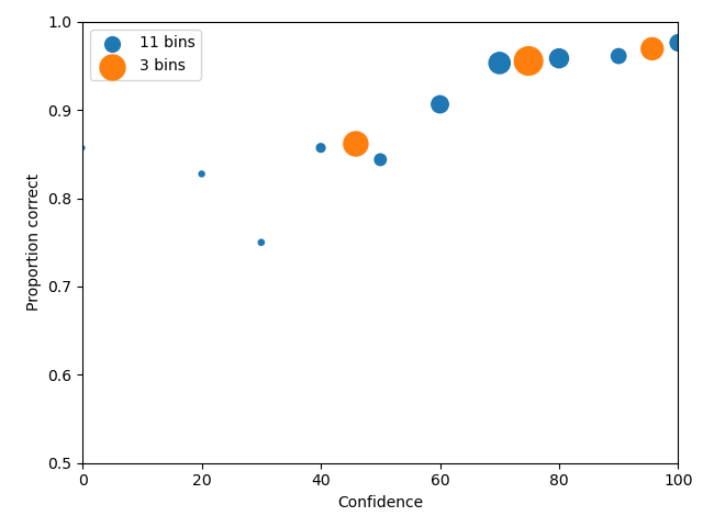
A good example is collapsing data, one might want to check the effect of rebinning the data. In the following example, the test1.csv is processed twice, once with the original binning (dr1 and dp1) and one with 3 confidence bins (dr2 and dp2)

• python
• R

import pyWitness
dr1 = pyWitness.DataRaw("test1.csv")
dr2 = pyWitness.DataRaw("test1.csv")

dr2.collapseContinuousData(column = "confidence",bins = [-1,60,80,100],labels=None)

dp1 = dr1.process()
dp2 = dr2.process()

dp1.plotCAC()
dp2.plotCAC()

pyw <- import("pyWitness")
dr1 <- pyw$DataRaw("./test1.csv")
dr2 <- pyw$DataRaw("./test1.csv")

dr2$collapseContinuousData(column = "confidence",bins = c(-1,60,80,100),labels=py_none())

dp1 <- dr1$process()
dp2 <- dr2$process()

dp1$plotCAC()
dp2$plotCAC()

Overlaying plots

In general, each plotXXX function does not create a canvas, so to overlay plots the functions need to be called sequentially in order.

To make a legend the plots need to be given a label. So this example is the same as the

• python
• R

import pyWitness
dr1 = pyWitness.DataRaw("test1.csv")
dr2 = pyWitness.DataRaw("test1.csv")

dr2.collapseContinuousData(column = "confidence",bins = [-1,60,80,100],labels=None)

dp1 = dr1.process()
dp2 = dr2.process()

dp1.plotCAC(label = "11 bins")
dp2.plotCAC(label = "3 bins")

import matplotlib.pyplot as _plt
_plt.legend()

pyw <- import("pyWitness")
dr1 <- pyw$DataRaw("./test1.csv")
dr2 <- pyw$DataRaw("./test1.csv")

dr2$collapseContinuousData(column = "confidence",bins = c(-1,60,80,100),labels=py_none())

dp1 <- dr1$process()
dp2 <- dr2$process()

dp1$plotCAC(label="11 bins")
dp2$plotCAC(label = "3 bins")


mpl$pyplot$legend()
invisible(mpl$pyplot$ylim(0.50,1.00))

After overlaying plots it maybe important to change the plot axis ranges this can be done with xlim and ylim

• python
• R

xlim(0,100)
ylim(0.50,1.00)

invisible(mpl$pyplot$xlim(0,100))
invisible(mpl$pyplot$ylim(0.50,1.0))

Generating data from signal detection model

Raw and processed data can be generated simply from a signal detection model.

• python
• R

import pyWitness
dr = pyWitness.DataRaw("test1.csv")
dr.collapseContinuousData(column = "confidence",bins = [-1,60,80,100],labels=None)
dp = dr.process()
mf = pyWitness.ModelFitIndependentObservation(dp, debug=True)
mf.setEqualVariance()
mf.fit()
dr1 = mf.generateRawData(nGenParticipants=10000)

pyw <- import("pyWitness")
dr <- pyw$DataRaw("./test1.csv")
dr$collapseContinuousData(column = "confidence",bins = c(-1,60,80,100),labels=py_none())
dp <- dr1$process()
mf <- pyw$ModelFitIndependentObservation(dp, debug=TRUE)
mf$setEqualVariance()
mf$fit()
dr1 = mf$generateRawData(nGenParticipants=10000)

dr1 is a DataRaw object and is simulated data for 10,000 participants. dr1 can be used for any pyWitness analysis so ROC, CAC, pAUC, etc. The raw data can also be written to disk to either preserve and/or share with colleagues.

• python
• R

dr1.writeCsv("fileName.csv")
dr1.writeExcel("fileName.xlsx")

dr1$writeCsv("./fileName.csv")
dr1$writeExcel("./fileName.xlsx")

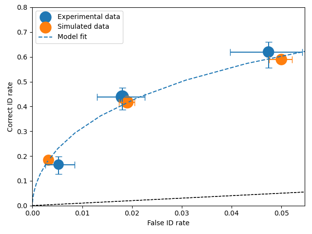
Having performed a fit on dr and generated dr1 a synthetic dataset

• python
• R

# Need to process the synthetic data
dp1 = dr1.process()

# calculate uncertainties using bootstrap
dp.calculateConfidenceBootstrap()
dp1.calculateConfidenceBootstrap()

# plot ROCs
dp.plotROC(label="Experimental data")
dp1.plotROC(label="Simulated data")
mf.plotROC(label="Model fit")

import matplotlib.pyplot as _plt
_plt.legend()

# Need to process the synthetic data
dp1 <- dr1$process()

# calculate uncertainties using bootstrap
dp$calculateConfidenceBootstrap()
dp1$calculateConfidenceBootstrap()

# plot ROCs
dp$plotROC(label="Experimental data")
dp1$plotROC(label="Simulated data")
mf$plotROC(label="Model fit")

mpl$pyplot$legend()
mpl$pyplot$show()

Power analysis

By having the ability to generate data from a model it is possible to vary the number of generated participants. This is not too dissimilar to bootstrapping. Instead of generating new samples (with replacement) from the data, new samples with variable numbers of participants is possible. For each sample all the analysis can be performed and dependence on sample size can be explored.

• python
• R

for nGen in numpy.linspace(500, 5000, 9+1) :
    drSimulated = mf.generateRawData(nGenParticipants = nGen)
    dpSimulated = drSimulated.process()
    dpSimulated.calculateConfidenceBootstrap(nBootstraps=2000)
    print(nGen, dpSimulated.liberalTargetAbsentSuspectId,dpSimulated.pAUC, dpSimulated.pAUC_low, dpSimulated.pAUC_high)

for (nGen in list(500,1000,1500)) {
    drSimulated <- mf$generateRawData(nGenParticipants = nGen)
    dpSimulated <- drSimulated$process()
    dpSimulated$calculateConfidenceBootstrap(nBootstraps=as.integer(2000))
    print(nGen, dpSimulated$liberalTargetAbsentSuspectId,dpSimulated$pAUC, dpSimulated$pAUC_low, dpSimulated$pAUC_high)
}